How bad is Huffman coding?
Have you wondered how much more data one can pack by migrating from Huffman coding algorithm to more efficient range coding or arithmetic coding algorithm? In today’s article, let’s get a rough sense of how much the improvement would be using a real data, and compare to the theoretical limit predicted by Shannon’s information theory.
Entropy coding compresses data by using fewer bits to symbols that occur with high probability and more bits to symbols that occur with less probability. Some of well-known entropy coding schemes include Huffman coding, arithmetic coding, and range coding. Since arithmetic coding and range coding are practically equivalent, let’s focus on the difference on Huffman vs range coding. In particular, we want to examine how much range coding improves upon Huffman coding.
Huffman coding encodes symbols into fixed codes while range coding encodes symbols in context. Range coding offers better compression ratio than Huffman coding when the probabilities are not exactly power of 2, but how much?
We will take the first 32kB block from linux.tar source code as our typical text data. For simplicity, let’s use a unigram model to calculate probabilities. Below is each (byte, count) for each symbol with non-zero probability in the 32kB block of the example data
(0, 5861)
(9, 2)
(10, 931)
(32, 2235)
(33, 10)
(34, 10)
(35, 80)
(36, 2)
(39, 1150)
(40, 9)
(41, 7)
(42, 64)
(44, 8)
(45, 624)
(46, 269)
(47, 63)
(48, 382)
(49, 62)
(50, 52)
(51, 20)
(52, 43)
(53, 33)
(54, 54)
(55, 11)
(56, 11)
(57, 5)
(58, 120)
(60, 82)
(61, 10)
(62, 82)
(63, 1)
(64, 82)
(65, 111)
(66, 57)
(67, 54)
(68, 21)
(69, 18)
(70, 16)
(71, 16)
(72, 5)
(73, 39)
(74, 3)
(75, 9)
(76, 40)
(77, 21)
(78, 19)
(79, 31)
(80, 42)
(81, 1)
(82, 16)
(83, 69)
(84, 24)
(85, 5)
(86, 6)
(87, 10)
(88, 3)
(89, 2)
(91, 14)
(92, 6)
(93, 14)
(94, 7)
(95, 2219)
(97, 1593)
(98, 219)
(99, 1204)
(100, 545)
(101, 2203)
(102, 942)
(103, 296)
(104, 811)
(105, 865)
(106, 24)
(107, 169)
(108, 726)
(109, 491)
(110, 974)
(111, 1401)
(112, 415)
(113, 40)
(114, 1621)
(115, 882)
(116, 1030)
(117, 377)
(118, 200)
(119, 85)
(120, 114)
(121, 229)
(122, 36)
(124, 2)
(126, 1)
The most frequent byte is 0x00 as tar appends a lot of these when concatenating files. We then convert the count to probability p by dividing by the total, 32768. For each symbol, we can calculate code length, which is -log2(p).
Theoretical Limit
Below shows (symbol, code_length). Notice the symbol 0x00 is encoded with 2.483 bits, while 0x09 is encoded with 14-bits. This is expected, as we want to use short codes for more frequent symbols and longer codes for infrequent symbols.
(0, 2.4830688780013035)
(9, 14.0)
(10, 5.137362642441206)
(32, 3.8739408839293197)
(33, 11.678071905112638)
(34, 11.678071905112638)
(35, 8.678071905112638)
(36, 14.0)
(39, 4.832581854168263)
(40, 11.830074998557688)
(41, 12.192645077942396)
(42, 9.0)
(44, 12.0)
(45, 5.714597781137751)
(46, 6.928537637443376)
(47, 9.022720076500084)
(48, 6.422571171964251)
(49, 9.045803689613125)
(50, 9.299560281858907)
(51, 10.678071905112638)
(52, 9.573735245297902)
(53, 9.955605880641546)
(54, 9.245112497836532)
(55, 11.540568381362704)
(56, 11.540568381362704)
(57, 12.678071905112638)
(58, 8.093109404391482)
(60, 8.642447995381916)
(61, 11.678071905112638)
(62, 8.642447995381916)
(63, 15.0)
(64, 8.642447995381916)
(65, 8.205584133649895)
(66, 9.167109985835259)
(67, 9.245112497836532)
(68, 10.60768257722124)
(69, 10.830074998557688)
(70, 11.0)
(71, 11.0)
(72, 12.678071905112638)
(73, 9.714597781137751)
(74, 13.415037499278844)
(75, 11.830074998557688)
(76, 9.678071905112638)
(77, 10.60768257722124)
(78, 10.752072486556415)
(79, 10.045803689613125)
(80, 9.60768257722124)
(81, 15.0)
(82, 11.0)
(83, 8.891475543221832)
(84, 10.415037499278844)
(85, 12.678071905112638)
(86, 12.415037499278844)
(87, 11.678071905112638)
(88, 13.415037499278844)
(89, 14.0)
(91, 11.192645077942396)
(92, 12.415037499278844)
(93, 11.192645077942396)
(94, 12.192645077942396)
(95, 3.8843060478029887)
(97, 4.36246944847469)
(98, 7.225212940398826)
(99, 4.766380323240298)
(100, 5.909887580335711)
(101, 3.8947462202991168)
(102, 5.120416750387217)
(103, 6.79054663437105)
(104, 5.336441895782727)
(105, 5.243443677475913)
(106, 10.415037499278844)
(107, 7.599120563717816)
(108, 5.496174262004249)
(109, 6.060420785685307)
(110, 5.0722220379176575)
(111, 4.547758759569182)
(112, 6.303032473765713)
(113, 9.678071905112638)
(114, 4.3373316244824585)
(115, 5.2153651544424795)
(116, 4.991571377929419)
(117, 6.4415792867313355)
(118, 7.356143810225276)
(119, 8.590609063862297)
(120, 8.167109985835259)
(121, 7.160796211903056)
(122, 9.830074998557688)
(124, 14.0)
(126, 15.0)
Finally, we can calculate the average number of bits per symbol, which is precisely entropy

Using log with base 2, we obtain entropy of 4.704 bits/symbol. Without compression, it would be 8-bits, so this gives us compression ratio of 1.7.
Multiplying by the number of symbols (32kB), we get 154138 bits or 19268 bytes. That is, we can compress 32768 bytes of data into at minimum 19268 bytes using a simple unigram model, achieving compression ratio of 1.7. This, by the way, assumes that the decoder already knows the probabilities of the incoming data. In practice, that information may not be known and may need to be transmitted as well, but for the sake of simplicity, let’s ignore that factor for now.
Huffman Coding
Now, let’s see how much compression Huffman coding can achieve. The following shows (symbol, code_length) of each symbols with non-zero probability.
(0, 3)
(9, 14)
(10, 5)
(32, 4)
(33, 12)
(34, 12)
(35, 9)
(36, 14)
(39, 5)
(40, 12)
(41, 12)
(42, 9)
(44, 12)
(45, 6)
(46, 7)
(47, 9)
(48, 6)
(49, 9)
(50, 9)
(51, 11)
(52, 9)
(53, 10)
(54, 9)
(55, 12)
(56, 11)
(57, 13)
(58, 8)
(60, 9)
(61, 12)
(62, 9)
(63, 15)
(64, 9)
(65, 8)
(66, 9)
(67, 9)
(68, 11)
(69, 11)
(70, 11)
(71, 11)
(72, 13)
(73, 10)
(74, 13)
(75, 12)
(76, 10)
(77, 10)
(78, 11)
(79, 10)
(80, 9)
(81, 15)
(82, 11)
(83, 9)
(84, 10)
(85, 13)
(86, 12)
(87, 12)
(88, 13)
(89, 14)
(91, 11)
(92, 12)
(93, 11)
(94, 12)
(95, 4)
(97, 4)
(98, 7)
(99, 5)
(100, 6)
(101, 4)
(102, 5)
(103, 7)
(104, 5)
(105, 5)
(106, 10)
(107, 8)
(108, 5)
(109, 6)
(110, 5)
(111, 4)
(112, 6)
(113, 10)
(114, 4)
(115, 5)
(116, 5)
(117, 7)
(118, 7)
(119, 9)
(120, 8)
(121, 7)
(122, 10)
(124, 14)
(126, 14)
Comparing the code length from the theoretical limit, we do see some inefficiencies, as we need to round up to the nearest integer. For example, symbol 0x00 is encoded with 3-bits, which is ~0.5bit more than its theoretical limit. Calculating for the total compressed data, we get 19417 bytes. This is only 149 more bytes compared to the theoretical limit, accounting less than 0.8% overhead. This is much better than my expectation.
Range Coding
Now, let’s see what we get from range coding. We expect it to fall in somewhere between the theoretical limit and the Huffman coding. Using the implementation described here, we get 19280 bytes, only 12 more byte than the theoretical limit. That is less than 0.07% overhead, which is 10x less overhead compared to Huffman coding.
Below summarizes our finding today
original data: 32768 bytes
huffman coded: 19417 bytes
range coded: 19280 bytes
theoretical limit: 19268 bytes
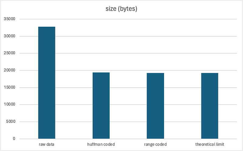
Obviously, the result can differ significantly depending on the data, but roughly speaking, the compression inefficiency introduced by Huffman coding seems to be quite insignificant, at less than 1%. Though range coding offers much less overhead, the compression ratio is about the same. So, my conclusion is that Huffman coding is quite good and can achieve compression ratio close to the theoretical limit.