Performance optimization — branchless programming
Everyone wants to write program that runs fast and efficient. Today, let’s have a look at one of the performance optimization techniques: branchless programming. We will go through an example where branchless optimization achieves whopping 7x faster performance! You can find the full source code here.
If you are not familiar with the topic yet, these two videos will serve as excellent introduction to the topic.
Branch misprediction overhead remains high in current processors due to deep pipelines and speculative execution, which cause significant time and resource waste when a misprediction occurs, despite advanced prediction techniques.
Branchful implementation
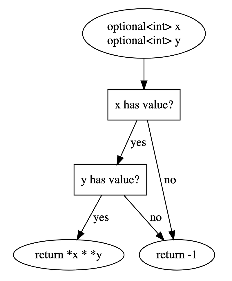
Branching means there are multiple paths of instructions for the program to execute. A classic example is with if/else and switch statements. Let’s say we have a function that takes in two optional<int> arguments. The function is to
- if both arguments contain values: compute the product and return
- else: return a preset value
A typical implementation would involve a simple if/else as below
int branchful(std::optional<int> x, std::optional<int> y) {
    const int NULL_VALUE = -1;

    if (x.has_value() && y.has_value()) {
        return *x * *y;
    } else {
        return NULL_VALUE;
    }
}
How many branches do we have in the code? Well, though not obvious, the answer is 2. The not-so-obvious branch comes from the logical AND operator &&.
Branchful control flow
Let’s examine the assembly code to verify. Below is what gcc produces without any optimization (so that the function is not inlined but even with -O2 flag, gcc still implements with branch instructions)
branchful(std::optional<int>, std::optional<int>):
    push    rbp
    mov     rbp, rsp
    push    rbx
    sub     rsp, 24
    mov     QWORD PTR [rbp-24], rdi
    mov     QWORD PTR [rbp-32], rsi
    lea     rax, [rbp-24]
    mov     rdi, rax
    call    std::optional<int>::has_value() const
    test    al, al
    je      .L12
    lea     rax, [rbp-32]
    mov     rdi, rax
    call    std::optional<int>::has_value() const
    test    al, al
    je      .L12
    mov     eax, 1
    jmp     .L13
.L12:
    mov     eax, 0
.L13:
    test    al, al
    je      .L14
    lea     rax, [rbp-24]
    mov     rdi, rax
    call    std::optional<int>::operator*() &
    mov     ebx, DWORD PTR [rax]
    lea     rax, [rbp-32]
    mov     rdi, rax
    call    std::optional<int>::operator*() &
    mov     eax, DWORD PTR [rax]
    imul    eax, ebx
    jmp     .L15
.L14:
    mov     eax, -1
.L15:
    mov     rbx, QWORD PTR [rbp-8]
    leave
    ret
We can find the je operation right after std::optional<int>::has_value() call for each argument. With this implementation, the benchmark program took 4.7s to complete.
Branchless implementations 1
How could we implement it without branching? One trick is to use array indexing. That is, prepare a lookup table that contains all possible values. Then, select the correct one from the table using the conditional variable.
int lookup_table(std::optional<int> x, std::optional<int> y) {
    const int NULL_VALUE = -1;

    // construct a lookup table of all possible values
    int options[2] = {NULL_VALUE, *x * *y};

    // construct the index from the conditional variable
    // note bitwise operation `&` and not logical operation `&&`
    auto ix = x.has_value() & y.has_value();

    // select and return
    return options[ix];
}
Let’s verify that there is no branching instruction from the assembly code generated by gcc.
lookup(std::optional<int>, std::optional<int>):
    push    rbp
    mov     rbp, rsp
    push    rbx
    sub     rsp, 40
    mov     QWORD PTR [rbp-40], rdi
    mov     QWORD PTR [rbp-48], rsi
    lea     rax, [rbp-40]
    mov     rdi, rax
    call    std::optional<int>::has_value() const
    movzx   ebx, al
    lea     rax, [rbp-48]
    mov     rdi, rax
    call    std::optional<int>::has_value() const
    movzx   eax, al
    and     eax, ebx
    mov     DWORD PTR [rbp-20], eax
    mov     QWORD PTR [rbp-28], 0
    mov     DWORD PTR [rbp-28], -1
    lea     rax, [rbp-40]
    mov     rdi, rax
    call    std::optional<int>::operator*() &
    mov     ebx, DWORD PTR [rax]
    lea     rax, [rbp-48]
    mov     rdi, rax
    call    std::optional<int>::operator*() &
    mov     eax, DWORD PTR [rax]
    imul    eax, ebx
    mov     DWORD PTR [rbp-24], eax
    mov     eax, DWORD PTR [rbp-20]
    cdqe
    mov     eax, DWORD PTR [rbp-28+rax*4]
    mov     rbx, QWORD PTR [rbp-8]
    leave
    ret
Viola! There is not a single branching instruction at all! The same benchmark program took 0.7s to complete—that is 6 times faster!
Branchless implementations 2
We are not done yet. There is another variant we could try. This time, we are going to magically compute the return value directly. This may well be faster than the lookup table approach because indexing operation from the lookup table approach is slow as it needs access to the memory.
Rather than creating the lookup table and indexing, we will use bit-mask approach. Given signed cond taking 0 or 1 boolean value, we could subtract 1 and get a conditional mask containing all-zero-bits vs all-one-bits. Then, we could perform bitwise operations to construct the value we want directly.
int bitmasking(std::optional<int> x, std::optional<int> y) {
    const int NULL_VALUE = -1;

    auto prod = *x * *y;
    int cond = x.has_value() & y.has_value();

    // either all-zero-bits or all-one-bits
    int mask = cond - 1;

    // bitmasking operations
    return (mask & NULL_VALUE) | (~mask & prod);
}
Let’s verify its assembly code.
bitmasking(std::optional<int>, std::optional<int>):
    push    rbp
    mov     rbp, rsp
    push    rbx
    sub     rsp, 40
    mov     QWORD PTR [rbp-40], rdi
    mov     QWORD PTR [rbp-48], rsi
    lea     rax, [rbp-40]
    mov     rdi, rax
    call    std::optional<int>::operator*() &
    mov     ebx, DWORD PTR [rax]
    lea     rax, [rbp-48]
    mov     rdi, rax
    call    std::optional<int>::operator*() &
    mov     eax, DWORD PTR [rax]
    imul    eax, ebx
    mov     DWORD PTR [rbp-20], eax
    lea     rax, [rbp-40]
    mov     rdi, rax
    call    std::optional<int>::has_value() const
    movzx   ebx, al
    lea     rax, [rbp-48]
    mov     rdi, rax
    call    std::optional<int>::has_value() const
    movzx   eax, al
    and     eax, ebx
    mov     DWORD PTR [rbp-24], eax
    mov     eax, DWORD PTR [rbp-24]
    sub     eax, 1
    mov     DWORD PTR [rbp-28], eax
    mov     eax, DWORD PTR [rbp-28]
    or      eax, DWORD PTR [rbp-20]
    mov     rbx, QWORD PTR [rbp-8]
    leave
    ret
Again, completely free of branching! This implementation ran in just 0.6s, resulting in 7x faster performance compared to the branchful implementation!
Profiling
Measuring the program’s runtime is one thing, but for more scientific analysis, we need to actually measure the branch-related instruction counts. For that, perf is the best tool.
perf stat -e instructions,branches,branch-misses command [args...]
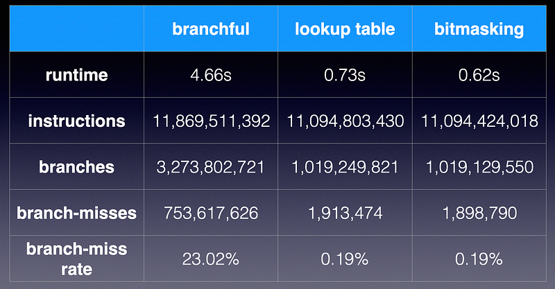
perf stat comparison
First, notice that the number instructions are very similar among all three implementations. The branchless implementations (lookup and bitmasking) reduce the branch instructions by 3x. More importantly, the branch-misses are reduced by impressive 400x with branchless implementations. This explains why we are seeing 7x speed up. The remaining branches are from other parts of the program, and their branch-miss rate is only 0.2%. This confirms our hypothesis that branch mispredictions were the culprit in slowing down the program. By the way, this measures the program when compiled by gcc with -O2 optimization.
Discussions
Note that we are actually doing more work with branchless implementations because we are performing the multiplication *x * *y regardless of the condition, as opposed to only when both arguments contain values in the branchful implementation. Typically, the branchless optimization works well if the branch misprediction cost is greater than the extra work we do. This implies that the branchless programming works well under these conditions
- data: close to random in which case branch prediction is very difficult
- workload: light extra work is required
- compiler: not so clever to do branchless optimization for us
For example, I obtained 7x performance gain when compiled with gcc but no gain when compiled with llvm , as llvm aggressively performs branchless optimization even for the branchful implementation.
Premature optimization is the root of all evil [Donald Knuth]
Please do not get the idea that we should avoid if/else as much possible. That is outright wrong conclusion. The truth is that it really depends on so many factors, such as compiler, optimization flags, programming language, operating system, CPU, and the code itself. Unless you are an expert in this area, you probably won’t be able to tell just from reading the code.
The best practice is to always profile and locate the hotspot first, and then measure and compare alternative implementations at the hotspot.